In this post, I want to explore the key RL architecture and software optimizations DeepSeek made to create Deepseek-R1. I’ll provide a brief introduction to the RL setup and explain how GRPO makes traditional algorithims much more efficient. At the end, I’ll provide a brief overview of how DeepSeek-R1 was trained. Talk given at Cambridge AI Safety Hub Members Meeting in February, slides available here.

---

Preliminaries

Transformers

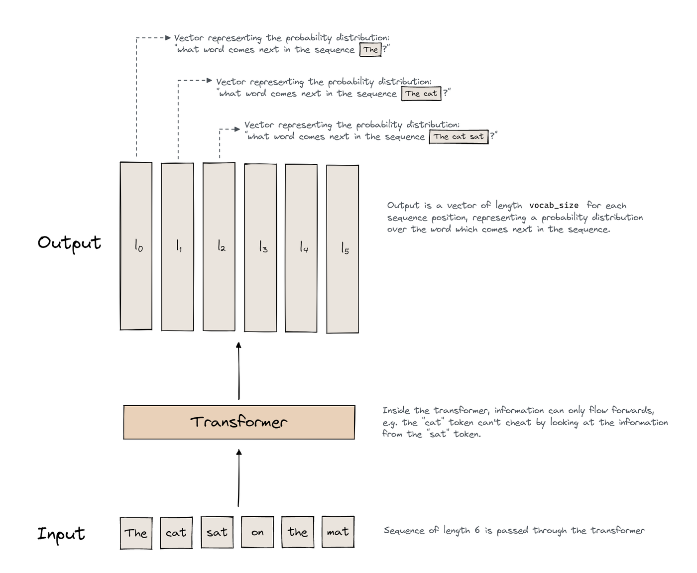
Modern transformers are autoregressive models. They predict the next token (essetially a word) given all the tokens before it:

$$p(x_1,\ldots,x_N) = \prod_{n=1}^N p(x_n|x_1,\ldots,x_{n-1})$$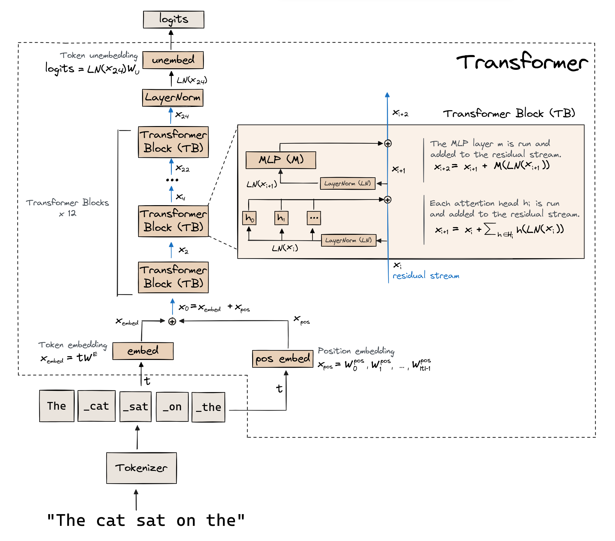

At a high level, input natural language are broken up into tokens, and converted to a numerical form. The output is then a probability distribution over the next possible token (from logits), and the next token is sampled from this distribution.

---

Reinforcement Learning

We provide a brief overview of the RL setup.

• An agent in state $s$ issues an action $a$ to the environment, and the environment replies with state, reward pairs $(s',r)$. We can then define a trajectory $\tau$ as a sequence of states and actions: $s_0, a_0, r_1, a_1, r_2, s_2, a_2, r_3...$

• The agent chooses actions using a policy $\pi$ which can either be a deterministic function $a=\pi(s)$ from states to actions, or more generally actions are sampled $a \sim \pi(\cdot|s)$

• The return at time $t$ is the sum of rewards obtained after time $t$ until the time $T$ when the terminal state is reached, discounted by how far into the future:

$$G_t = \sum_{k=0}^{\infty} \gamma^k r_{t+k+1} = r_{t+1} + \gamma r_{t+2} + \gamma^2 r_{t+3} ...$$

• The state value function $V_\pi(s)$ is the expected return, if you start in state $s$ and always act according to policy $\pi$:

  $$V_{\pi}(s) = \mathbb{E}_{\pi}\left[G_t| s_t = s\right]$$

We deal with these core quantities:

• The action value function is the expected return if you start in state $s$, take an arbitrary action $a$ (which may not have come from the policy), and then afterwards forever act according to policy $\pi$:

  $$Q_\pi(s, a) = \mathbb{E}_{\pi} \left[G_t| s_t = s, a_t = a\right]$$

• The advantage function describes how much better it is to take a specific action $a$ in state $s$, over randomly selecting an action according to $\pi(\cdot|s)$, assuming you act according to $\pi$ forever after:

  $$A_\pi(s, a) = Q_\pi(s, a) - V_\pi(s)$$

Trust Region Policy Optimization (TRPO)

Let $\pi_\theta$ denote a policy with parameters $\theta$. We aim to maximize the expected return $J$ of policy $\pi_\theta$, where we take expectation over all possible trajectories $\tau$ generated by following policy $\pi_\theta$

$$J(\pi_\theta) = \underset{\tau \sim \pi_\theta}{\mathbb{E}}[G(\tau)]$$

To achieve the optimum $\pi_\theta$ that maximizes J, we can iteratively update $\pi_{\theta_{k}}$ according to:

$$\theta_{k+1} = \arg \max_\theta \mathcal{L}(\theta_k, \theta) = \arg \max_\theta \underset{s,a\sim\pi_{\theta_k}}{\mathbb{E}} \left[L(s, a, \theta_k, \theta)\right], \quad \text{s.t. } \bar{D}_{KL}(\theta\|\theta_k) \leq \delta$$

where $\mathcal{L}(\theta_k, \theta)$ is the surrogate advantage, a measure of how policy $\pi_\theta$ performs relative to the old policy $\pi_{\theta_k}$ using data from the old policy:

$$L(s, a, \theta_k, \theta) = \frac{\pi_\theta(a|s)}{\pi_{\theta_k}(a|s)} A_{\pi_{\theta_k}}(s,a)$$

TRPO updates policies by taking the largest step possible to improve performance, while satisfying a special constraint on how close the new and old policies are allowed to be.

Proximal Policy Optimization (PPO)

Proximal Policy Optimization updates policies via:

$$\theta_{k+1} = \arg \max_\theta \mathcal{L}(\theta_k, \theta) = \arg \max_\theta \underset{s,a\sim\pi_{\theta_k}}{\mathbb{E}} \left[L(s, a, \theta_k, \theta)\right]$$

typically taking multiple steps of SGD to maximize the objective. Here $L$ is given by:

$$L(s, a, \theta_k, \theta) = \min\Bigg(\frac{\pi_\theta(a|s)}{\pi_{\theta_k}(a|s)}A_{\pi_{\theta_k}}(s,a), \text{clip}\left(\frac{\pi_\theta(a|s)}{\pi_{\theta_k}(a|s)}, 1-\epsilon, 1+\epsilon\right)A_{\pi_{\theta_k}}(s,a)\Bigg)$$

PPO-Clip doesn’t have a KL-divergence term in the objective and doesn’t have a constraint at all. Instead relies on specialized clipping in the objective function to remove incentives for the new policy to get far from the old policy.

Generalized Advantage Estimation (GAE) is used in PPO to estimate the advantage function:

$$A_t = \sum_{l=0}^{\infty} (\gamma \lambda)^l \delta_{t+l} \\ = \delta_t + (\gamma \lambda) \delta_{t+1} + (\gamma \lambda)^2 \delta_{t+2} + \dots$$

where:

• $\delta_t = r_t + \gamma V(s_{t+1}) - V(s_t)$ (TD error)

  • the reward $r_t$ is usually given by a trained (neural) reward model

• $\gamma$ is the discount factor

• $\lambda$ is the GAE parameter (tradeoff between bias and variance)

• $V(s)$ is the value function estimate, from value network

  • Often a value network $V_\psi$ needs to be trained alongside the policy model $\pi_\theta$ to estimate the value, often as big as the policy model itself

General RL Training Setup

Objective:

$$J(\pi_\theta) = \mathbb{E}_{\tau \sim \pi_\theta}\left[\sum_{t=0}^{T} \gamma^t r_t\right]$$

where $\tau = \{s_0, a_0, r_1, s_1, a_1, \dots, s_T\}$ is a trajectory. For LLMs, actions $a_t$ here are tokens!

Policy Gradient:

$$\nabla_\theta J(\pi_\theta) = \mathbb{E}_{s,a \sim \pi_\theta}\left[\nabla_\theta \log \pi_\theta(a|s) \, Q^{\pi_\theta}(s,a)\right]$$

or equivalently, using the advantage function $A^{\pi_\theta}(s,a)$:

$$\nabla_\theta J(\pi_\theta) = \mathbb{E}_{s,a \sim \pi_\theta}\left[\nabla_\theta \log \pi_\theta(a|s) \, A^{\pi_\theta}(s,a)\right]$$

Trajectory Collection: LLM interacts with the environment (reward model) to sample trajectories. For each timestep:

$$s_t \xrightarrow{\pi_\theta} a_t \rightarrow r_{t+1},\, s_{t+1}$$

Return and Advantage Calculation:

$$G_t = \sum_{k=0}^{\infty} \gamma^k r_{t+k+1}, \quad A(s_t,a_t) = Q^{\pi_\theta}(s_t,a_t) - V^{\pi_\theta}(s_t)$$

Generalized Advantage Estimation (GAE) are used to compute $A(s_t,a_t)$ practically

Policy Update:

$$\theta_{k+1} = \theta_k + \alpha\, \nabla_\theta J(\pi_\theta)$$

Using the computed advantages, update the policy parameters and value network by maximizing a surrogate objective (e.g., the PPO objective) to favor actions with higher expected returns. Repeat until agent’s performance converges.

---

R1-Zero

Group Relative Policy Optimization (GRPO)

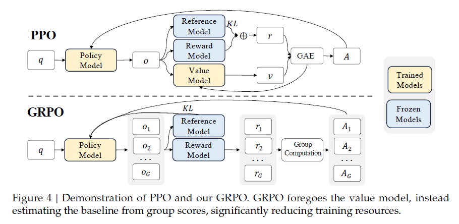
DeepSeek uses GRPO (created in-house) which foregoes the value network and estimates the advantages directly from group rewards instead.

For each question $q$, GRPO samples a group of outputs $\{o_i\}_{i=1}^G$ from the old policy $\pi_{\theta_{\text{old}}}$ and then optimizes the policy model $\pi_\theta$ by maximizing:

$$\begin{aligned} \mathcal{J}_{\text{GRPO}}(\theta) &= \mathbb{E}[q \sim P(Q), \{o_i\}_{i=1}^G \sim \pi_{\theta_{\text{old}}}(Q|q)] \\ &\quad \cdot \frac{1}{G}\sum_{i=1}^G\left(\min\left(\frac{\pi_\theta(o_i|q)}{\pi_{\theta_{\text{old}}}(o_i|q)}A_i, \text{clip}\left(\frac{\pi_\theta(o_i|q)}{\pi_{\theta_{\text{old}}}(o_i|q)}, 1-\epsilon, 1+\epsilon\right)A_i\right) - \beta\mathbb{D}_{KL}(\pi_\theta\|\pi_{\text{ref}})\right) \end{aligned}$$$$\mathbb{D}_{KL}(\pi_\theta\|\pi_{\text{ref}}) = \frac{\pi_{\text{ref}}(o_i|q)}{\pi_\theta(o_i|q)} - \log\frac{\pi_{\text{ref}}(o_i|q)}{\pi_\theta(o_i|q)} - 1$$

where $\epsilon$ and $\beta$ are hyper-parameters, and $A_i$ is the advantage ¹

GRPO Advantages

Advantages $A_i$ are computed using group rewards $\{r_1,r_2,\ldots,r_G\}$:

$$A_i = \frac{r_i - \text{mean}(\{r_1,r_2,\ldots,r_G\})}{\text{std}(\{r_1,r_2,\ldots,r_G\})} $$

As the value network is typically another model of comparable size as the policy model, it brings a substantial memory and computational burden. GRPO eliminates value network completely, saving enourmous amounts of compute!

Reward Modelling

R1-Zero uses a rule-based reward system consisting of:

• Accuracy rewards: The accuracy reward model evaluates whether the response is correct.
  • For math problems with deterministic results, can easily check if right or wrong. Provider higher reward if right.
  • For LeetCode problems, a compiler can be used to generate feedback based on predefined test cases
• Format rewards: Enforces the model to put its thinking process between <think> and </think> tags.

Usually for LLMs, a neural reward model (neural network used to estimate rewards) is used to provide rewards, as human preferences or requirements are difficult to define in a rules-based way. However, R1 does not use any neural reward model:

• Neural reward model may suffer from reward hacking

• Retraining the reward model needs additional training resources and it complicates the whole training pipeline

Performance

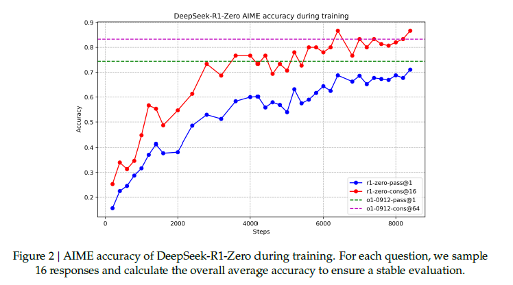
There’s no supervised fine tuning involved at all in R1-Zero, which is extremely impressive considering its performance. Majority voting bring performance on AIME benchmark from 71% to 86%.

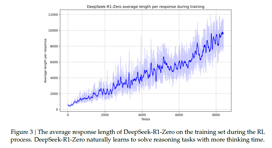
R1-Zero naturally acquires the ability to solve increasingly complex reasoning tasks by leveraging extended test-time computation (increased Chain-Of-Thought length). Behaviours like backtracking and reflection naturally emerge, which is absolutely incredible…

Problems

R1-Zero exhibits poor readability of its chain of thoughts, where language mixing often occurs. I suspect this is probably some form of reward over-optimization, as it is more efficient to reason in its own language and achieve higher reward.

We know different languages have different information density. This can be thought of as the “efficiency” of language, given a constraint on its length. Suppose an LLM had a length constraint (the context window), and was incentivised to achieve a goal. Won’t you expect the LLM to naturally use more information dense languages? Or even more extreme - if it were intelligent enough - create its own language that is information dense enough to achieve its goals?

I worry about this aspect quite abit, about future intelligent systems reasoning in its own language uninterpretable to humans. If you’ve ever seen Villeneuve’s incredible film Arrival, you would have seen the heptapods’ non-linear language which isn’t formed by sequentially combining words linearly. If these systems start communicating in their own language and are given goals by humans, you can see how this could cause all sorts of various problems.

---

R1 Training Pipeline

Phase 1: Cold Start

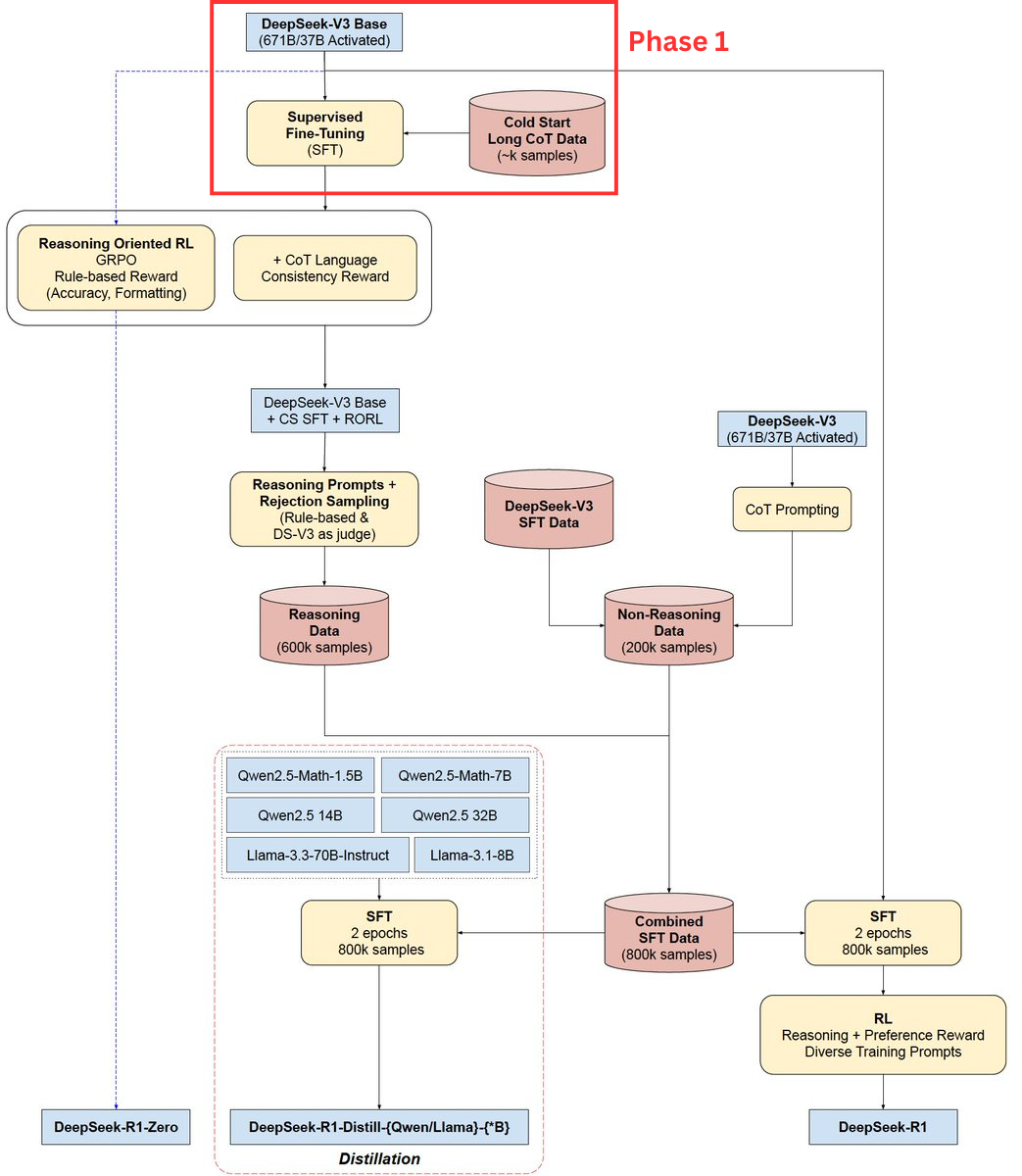
• Construct and collect small amounts (thousands) of long CoT data to fine-tune V3
  • Using few-shot prompting on V3 with long CoT examples
  • Direct prompting on V3 for detailed answers with reflection
  • Gathering DeepSeek-R1-Zero outputs with human post-processing
• Key advantages:
  • Readability: R1-Zero has unreadable responses. We define output format as |special_token|<reasoning_process>|special_token|<summary> so reasoning process (CoT) and summary of reasoning provided
  • Potential: Carefully designed patterns with human priors show better performance vs R1-Zero

Phase 2: Reasoning Reinforcement Learning

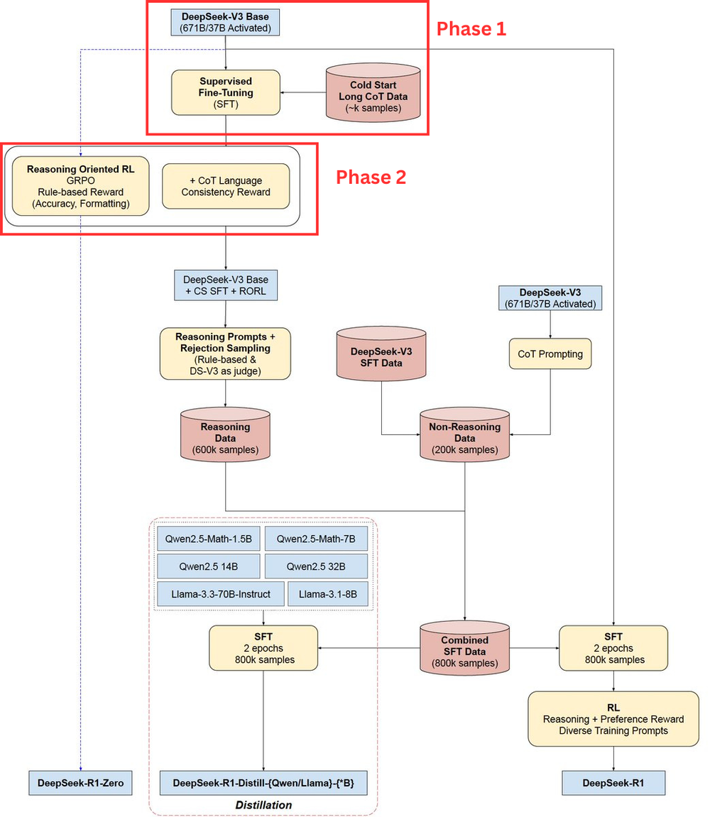
After cold start fine-tuning, apply large-scale RL training similar to DeepSeek-R1-Zero:

• Focus on reasoning-intensive tasks:
  • Coding, mathematics, science, logic reasoning
  • Well-defined problems with clear solutions
• Language Consistency:
  • CoT exhibits language mixing in multi-language prompts
  • Introduce language consistency reward, measured as proportion of target language words in CoT

Final reward function combines reasoning task accuracy, language consistency reward, and formatting reward to train until convergence.

Phase 3: Rejection Sampling and Supervised Fine-Tuning

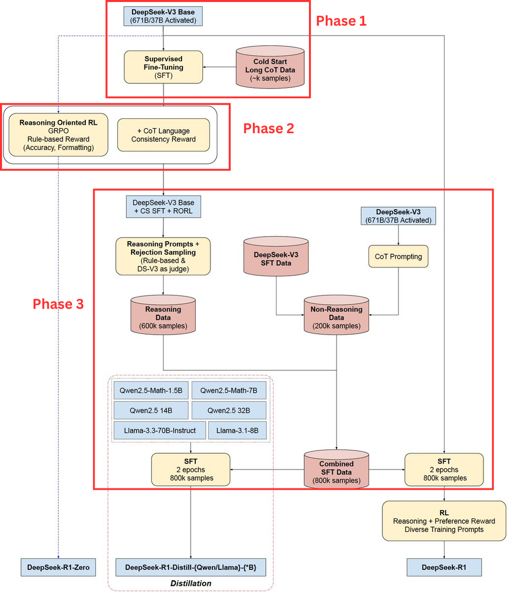
After RL convergence, collect SFT data from checkpoint for further training. Data includes:

Reasoning Data (600k samples)

• Rejection sampling from RL checkpoint
• Expanded dataset includes:
  • Rule-based rewards
  • Generative rewards via DeepSeek-V3 as LLM-Judge
• Quality filters:
  • Remove mixed languages
  • Filter long paragraphs
  • Remove chaotic code blocks

Non-Reasoning Data (200k samples)

• Types:
  • Writing
  • Factual QA
  • Self-cognition
  • Translation
• Reuse SFT data for DeepSeek-V3

Final fine-tuning on DeepSeek-V3-Base: 2 epochs on combined 800k samples

Phase 4: Diverse Reinforcement Learning Phase

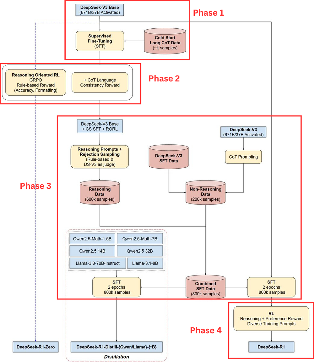
Secondary RL stage to align with human preferences while improving, helpfulnes, harmlessness, and reasoning:

Training Approach

• Reasoning data:
  • Same approach as DeepSeek-R1-Zero
  • Rule-based rewards on Math, code, logical reasoning
• General data:
  • Reward model as in DeepSeek V3
  • Use preference pairs

Helpful Honest Harmless (HHH) Criteria

• Helpfulness:
  • Focus on final summary in summary tag is useful and relevance
  • Preserves reasoning process in the reasoning tag
• Harmlessness:
  • Evaluate full response for potential biases or hamful content

---

R1 Engineering Unlocks

The DeepSeek team also did some insane software and hardware optimizations:

• Multi-Head Latent Attention (for efficient inference)
  • Low-rank join compression for K,Q,V matrices to reduce key-value cache memory usage
• DeepSeekMoE with Auxiliary-Loss-Free Load Balancing (efficient training)
  • 671B parameters, but only which 37B are activated for each token
• Multi-Token Prediction Objective

---

Conclusion

I think the core reason behind R1’s success was its sheer efficiency: getting rid of the value network via simple advantage estimation, using a simple reward model instead of a neural reward model, and all the hardware/software optimizations. The multi-phase training approach, while quite hacky, preserves the reasoning ability of R1-Zero while ensuring readability. All in all I’m very impressed by the DeepSeek team, and I hope you learnt something from this post!

---

References

Shao, Z., Wang, P., Zhu, Q., Xu, R., Song, J., Bi, X., Zhang, H., Zhang, M., Li, Y. K., Wu, Y., & Guo, D. (2024). DeepSeekMath: Pushing the Limits of Mathematical Reasoning in Open Language Models. arXiv:2402.03300 [cs.CL]. https://arxiv.org/abs/2402.03300

DeepSeek-AI, Guo, D., Yang, D., Zhang, H., Song, J., Zhang, R., Xu, R., Zhu, Q., Ma, S., Wang, P., et al. (2025). DeepSeek-R1: Incentivizing Reasoning Capability in LLMs via Reinforcement Learning. arXiv:2501.12948 [cs.CL]. https://arxiv.org/abs/2501.12948

DeepSeek-AI, Liu, A., Feng, B., Xue, B., Wang, B., Wu, B., Lu, C., Zhao, C., Deng, C., Zhang, C., et al. (2025). DeepSeek-V3 Technical Report. arXiv:2412.19437 [cs.CL]. https://arxiv.org/abs/2412.19437

ARENA curriculum. Transformer from Scratch. https://arena-chapter1-transformer-interp.streamlit.app/[1.1]_Transformer_from_Scratch

---