The Discrete Fourier Transform and Fast Fourier Transform
We analyze 1 the theoretical properties of both the Discrete Fourier Transform (DFT) and the optimized Fast Fourier Transform (FFT), and estimate their algorithmic complexity.
All code available on Github. Slides available here.
Discrete Fourier Transform
Theory
The DFT converts a finite-length time-domain signal into its frequency-domain representation. For an input signal $x[n]$ of length $N$, where $0 \le n \le N-1$, the DFT is defined as:
$$ X[k] = \sum_{n=0}^{N-1} x[n]\, W_N^{nk}, \quad 0 \le k \le N-1 \label{eq:DFT} $$where $W_N=e^{-j\frac{2\pi}{N}}$ is the $N$-th principal root of unity, and $X[k]$ is component at frequency $kf_s/N$ with sampling frequency $f_s$. We can rewrite $X[k]$ as an inner product:
$$ \begin{align} X[k] &= \left[ 1 \quad e^{-j\frac{2\pi k}{N}} \quad \ldots \quad e^{-j\frac{2\pi k}{N}(N-1)} \right] \begin{bmatrix} x[0] \\ x[1] \\ \vdots \\ x[N-1] \end{bmatrix} \\ &= \left[ 1 \quad W_N^k \quad \ldots \quad W_N^{(N-1)k} \right] \begin{bmatrix} x[0] \\ x[1] \\ \vdots \\ x[N-1] \end{bmatrix} \end{align} $$By varying $k$ from $0$ to $N-1$, we can collate all outputs ${X[k]}$ into a vector $\mathbf{X}$, collate all inputs $x[n]$ into a vector $\mathbf{x}$, to get:
$$ \mathbf{X}=\mathbf{W}\mathbf{x}, \quad \mathbf{W} = \begin{bmatrix} 1 & 1 & 1 & \cdots & 1 \\ 1 & W_N & W_N^2 & \cdots & W_N^{N-1} \\ 1 & W_N^2 & W_N^4 & \cdots & W_N^{2(N-1)} \\ \vdots & \vdots & \vdots & \ddots & \vdots \\ 1 & W_N^{N-1} & W_N^{2(N-1)} & \cdots & W_N^{(N-1)(N-1)} \end{bmatrix} $$where $\mathbf{W}$ is the DFT matrix.
Complexity
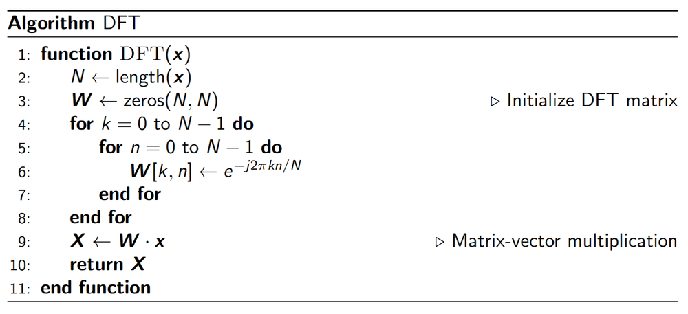
Direct implementation in MATLAB:
function X = dft_loop(x)
% Compute the Discrete Fourier Transform (DFT) of input vector x using naive loops
% x : input signal (vector)
% X : DFT of x

    % Convert input to a column vector for consistency
    x = x(:);
    N = length(x);       % Number of samples in the signal

    % Pre-allocate the output vector for efficiency
    X = zeros(N, 1);

    % Loop over each frequency bin k (from 0 to N-1)
    for k = 0:N-1
        sum_val = 0;
        % Loop over each time sample n (from 0 to N-1)
        for n = 0:N-1
            % Compute and accumulate the contribution for the k-th frequency component
            sum_val = sum_val + x(n+1) * exp(-1j * 2 * pi * k * n / N);
        end
        % MATLAB uses one-based indexing, so assign to X(k+1)
        X(k+1) = sum_val;
    end

end
MATLAB code (vectorized):
function X = dft_vectorized(x)
% Compute the Discrete Fourier Transform (DFT) of input vector x using vectorized operations
% x : input signal (vector)
% X : DFT of x

    % Convert input to a column vector for consistency
    x = x(:);
    N = length(x);       % Number of samples in the signal

    % Create index vectors: n as a row vector and k as a column vector
    n = 0:N-1;           % Time indices (row vector)
    k = n';              % Frequency indices (column vector)

    % Construct the DFT matrix using the formula: exp(-1j*2*pi*k*n/N)
    W = exp(-1j * 2 * pi * k * n / N);

    % Multiply the DFT matrix with the signal to obtain the transform
    X = W * x;

end
Direct computation of $\mathbf{X}$ requires $(N-1)^2$ complex multiplications and $N(N-1)$ complex additions. Since multiplication is more compute-intensive than addition, the asymptotic complexity is dominated by multiplication, giving $O(N^2)$.
Fast Fourier Transform
Preliminaries
We layout some properties of $W_N$ we’ll be using later
Property 1:
$$ W_N^2 = W_{N/2} $$Proof:
$$ W_N^2 = e^{-j\frac{2\pi}{N}\cdot 2} = e^{-j\frac{2\pi}{N/2}} = W_{N/2} $$More generally, $W_N^{2nk} = W_{N/2}^{nk}$.
Property 2:
$$ W_N^{k+\frac{N}{2}} = -W_N^k $$Proof:
$$ W_N^{k+\frac{N}{2}} = e^{-j\frac{2\pi}{N}\left(k+\frac{N}{2}\right)} = e^{-j\frac{2\pi}{N}k} \cdot e^{-j\pi} = -W_N^k $$Theory
The radix-2 FFT algorithms work by dividing the DFT into 2 DFTs of length $N/2$ each, and iterating. We introduce the simplest variant, called the Decimation-In-Time (DIT) algorithm.
Consider a $N$-point signal $x[n]$ of even length, indexed from $0$ to $N-1$. The derivation of the DIT radix-2 FFT begins by splitting the $x[n]$ into two parts — one part for the even-indexed values $x[2n]$ and one part for the odd-indexed values $x[2n + 1]$. Define two $N/2$-point signals $x_{even}[n]$ and $x_{odd}[n]$ as
$$x_{even}[n] = x[2n], \quad x_{odd}[n] = x[2n + 1], \quad 0 \leq n \leq N/2-1$$The DFT can be written as
$$ \begin{aligned} X[k] &= \sum_{n=0 \atop n \text{ even}}^{N-1} x[n] W_N^{nk} + \sum_{n=0 \atop n \text{ odd}}^{N-1} x[n] W_N^{nk}\\ &= \sum_{n=0}^{N/2-1} x[2n] W_N^{2nk} + \sum_{n=0}^{N/2-1} x[2n + 1] W_N^{(2n+1)k}\\ &= \sum_{n=0}^{N/2-1} x_{even}[n] W_N^{2nk} + \sum_{n=0}^{N/2-1} x_{odd}[n] W_N^{(2n+1)k} \\ &= \sum_{n=0}^{N/2-1} x_{even}[n] W_N^{2nk} + W_N^{k} \cdot \sum_{n=0}^{N/2-1} x_{odd}[n] W_N^{2nk}\\ \end{aligned} $$Noting that $W_N^{2}=W_{N/2}$ or more generally $W_N^{2nk}=W_{N/2}^{nk}$ , then
$$ \begin{aligned} X[k]&= \sum_{n=0}^{N/2-1} x_{even}[n] W_{N/2}^{nk} + W_N^{k} \cdot \sum_{n=0}^{N/2-1} x_{odd}[n] W_{N/2}^{nk} \end{aligned} $$Recognizing that the $\frac{N}{2}$-point DFT of $x_{even}[n]$ and $x_{odd}[n]$ are given by:
$$X_{even}[k] = \text{DFT}_{\frac{N}{2}}\{x_{even}[n]\} = \sum_{n=0}^{N/2-1} x_{even}[n] W_{N/2}^{nk}$$$$X_{odd}[k] = \text{DFT}_{\frac{N}{2}}\{x_{odd}[n]\} = \sum_{n=0}^{N/2-1} x_{odd}[n] W_{N/2}^{nk}$$we then obtain our core recursive equation:
$$ X[k] = X_{even}[k] + W_N^{k} \cdot X_{odd}[k] \label{eq:fft_int} $$Since $x_{even}[n]$ and $x_{odd}[n]$ are $N/2$-point signals with $0 \leq n \leq N/2-1$, their DFT are also only $N/2$-point signals. However, we require $0 \le k \le N-1$. We resolve this by noting their DFT coefficients are periodic with a period of $\frac{N}{2}$:
$$X_{even}[k] = X_{even}\left[k + \frac{N}{2}\right], \quad X_{odd}[k] = X_{odd}\left[k + \frac{N}{2}\right]$$This gives us
$$ X[k] = \begin{cases} X_{even}[k] + W_N^{k} \cdot X_{odd}[k], & \text{for } k = 0,1,\ldots,\frac{N}{2}-1 \\ X_{even}\left[k-\frac{N}{2}\right] + W_N^{k} \cdot X_{odd}\left[k-\frac{N}{2}\right], & \text{for } k = \frac{N}{2},\frac{N}{2}+1,\ldots,N-1 \end{cases} $$Noting $W_N^{k +\frac{N}{2}}=-W_{N}^{k}$, we write
$$ X[k] = \begin{cases} X_{even}[k] + W_N^{k} \cdot X_{odd}[k], & \text{for } k = 0,1,\ldots,\frac{N}{2}-1 \\ X_{even}\left[k-\frac{N}{2}\right] - W_N^{k-\frac{N}{2}} \cdot X_{odd}\left[k-\frac{N}{2}\right], & \text{for } k = \frac{N}{2},\frac{N}{2}+1,\ldots,N-1 \end{cases} $$finally giving us
$$ \begin{aligned} X[k] &= X_{even}[k] + W_N^{k} \cdot X_{odd}[k] \quad \text{for } 0 \leq k \leq \frac{N}{2} - 1 \\ X[k + N/2] &= X_{even}[k] - W_N^{k} \cdot X_{odd}[k] \quad \text{for } 0 \leq k \leq \frac{N}{2} - 1 \label{eq:fft_final} \end{aligned} $$The multipliers $W_N^k$ are known as twiddle factors. The first computation with $+W_N^k$ give us the first half of the full DFT vector $\mathbf{X}$, while the second computation with $-W_N^k$ give us the second half of $\mathbf{X}$.
Complexity
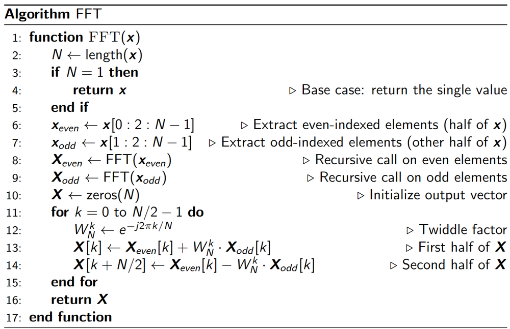
MATLAB code for FFT:
function X = fft_vectorized(x)
% computes the radix-2 FFT recursively using vectorized operations.
% If the length of x is not a power of 2, it is zero-padded to the next power of 2, added at the end

    x = x(:);         % Ensure x is a column vector
    N = length(x);

    % If N is not a power of 2, zero-pad x to the next power of 2
    M = 2^nextpow2(N);  % nextpow2 returns the exponent so that 2^exponent >= N
    if M ~= N
        %add zeros to the end
        x = [x; zeros(M - N, 1)];
        N = M;  % Update N to the new length
    end

    % Base case: if the input length is 1, return x
    if N == 1
        X = x;
        return;
    end

    % Recursively compute FFT for even and odd indices
    X_even = fft_vectorized(x(1:2:end)); %select all the even indices
    X_odd  = fft_vectorized(x(2:2:end)); % selects all the odd indices

    % Compute twiddle factors (complex exponentials) in a vectorized manner
    % row array
    factor = exp(-1j * 2 * pi * (0:N/2-1).' / N);

    % Combine the FFTs of the even and odd parts using the butterfly operation
    X = [X_even + factor .* X_odd;
         X_even - factor .* X_odd];

end
We can follow the above procedure to split an $N$-point DFT into two $\frac{N}{2}$-point DFT, giving us the above algorithim. Let $A_c(N)$ and $M_c(N)$ denote respectively the number of complex additions and multiplications for computing the DFT of an $N$-point complex sequence $x[n]$. Let $N$ be a power of 2, $N = 2^k$. Then, we have
$$A_c(N) = 2 A_c(N/2) + N \quad , \quad M_c(N) = 2 M_c(N/2) + \frac{N}{2} - 1$$as $N$ complex additions (addition of even and odd terms) and $\frac{N}{2} - 1$ complex multiplications ($W_N^{k} \cdot X_{odd}[k]$) are required to put the two $N/2$-point DFTs together. Note that a 2-point DFT is simply a sum and difference
$$X[0] = x[0] + x[1] , \quad X[1] = x[0] - x[1]$$Hence, the starting conditions are $A_c(2) = 2$ and $M_c(2) = 0$. Solving the recursive equation yields
$$A_c(N) = N \log_2 N \quad , \quad M_c(N) = \frac{N}{2} \log_2 N - N + 1$$Our overall complexity is $O(N\log N)$.
Experiments
Complexity
| Algorithm | O(N) | O(N²) | O(N³) | O(log N) | O(N log N) |
|---|---|---|---|---|---|
| my-DFT | 0.9208 | 0.9999 | 0.9864 | 0.4167 | 0.9417 |
| my-FFT | 0.9830 | 0.9657 | 0.9161 | 0.5634 | 0.9894 |
| MATLAB-FFT | 0.8491 | 0.7141 | 0.6526 | 0.8537 | 0.8287 |
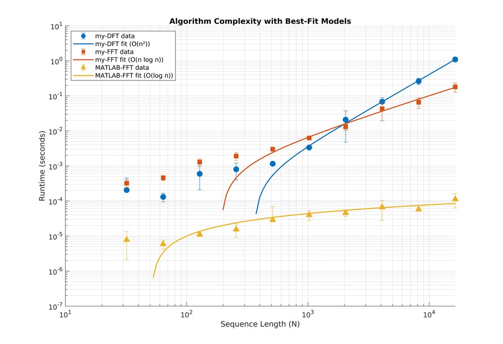
To verify the theoretical complexity, we measured the execution time for
computing the DFT over a range of signal lengths. For each signal length
$N$, $N$ samples were taken from a 5Hz sine wave, and the DFT/FFT
computation time recorded. We compare our implementation of DFT my-DFT, our implementation of FFT as my-FFT, and the MATLAB FFT implementation as MATLAB-FFT. You can view the measured execution times above on a
log-log plot. The FFT results clearly exhibit an $O(N\log N)$ scaling,
while the DFT scales as $O(N^2)$. These experimental results confirm the
significant computational advantage of using the FFT for large-scale
problems. We also note the much more efficient implementation of
MATLAB FFT, which uses the FFTW 2 package. The table above also shows the how
well different models fit to data. Both FFT implementations fit well to
$O(N)$ and $O(N\log N)$ models.
Numerical Error
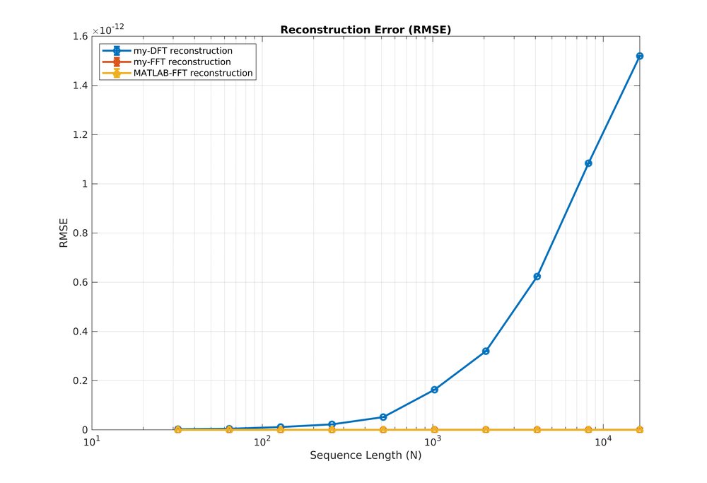
We evaluate numerical accuracy of above algorithims by
measuring reconstruction error of the reconstructed signal
$\text{RMSE} = \sqrt{\frac{1}{N}\sum_{i=1}^{N}|x_i - \hat{x}_i|^2}$
where $x_i$ is the original signal and $\hat{x}_i$ is the reconstructed
signal (using the MATLAB Inverse DFT function) Despite all errors
falling within the $10^{-12}$ range, indicating high overall accuracy,
the custom DFT implementation exhibits exponentially growing error with
increasing sequence length. In contrast, both FFT implementations
maintain consistently minimal error across all tested sequence lengths.
The superior numerical stability of FFT algorithms is possibly due to
its lower operation count (lower algorithmic complexity). Floating-point
rounding errors accumulate more significantly in DFT.
Conclusion
We study the theoretical motivations behind FFT. We verify that the computational complexity of the direct DFT implementation scales as $O(N^2)$, whereas our FFT implementation achieved the expected $O(N \log N)$ complexity, offering a significant improvement in efficiency.
References
Golub, G. H., & Van Loan, C. F. (1996). Matrix computations (3rd ed.). Johns Hopkins University Press.
Strang, G. (2007). Computational Science and Engineering. Wellesley-Cambridge Press. https://epubs.siam.org/doi/abs/10.1137/1.9780961408817
Ramalingam, C.S. Introduction to the Fast-Fourier Transform (FFT) Algorithm. https://www.ee.iitm.ac.in/~csr/teaching/pg_dsp/lecnotes/fft.pdf
Fast Fourier Transform (FFT). NYU Engineering. https://eeweb.engineering.nyu.edu/iselesni/EL713/zoom/fft